Post-Analysis for Modeling Tuning Experiments

Overview

Teaching: 15 min
Exercises: 50 min

Questions

How should we visualize the outputs from the post-processing phase?

What general trends do we observe from the last epoch results?

Objectives

Understand the effect of tuning the different hyperparameters.

Acquiring the art and common sense of the hyperparameter tuning.

Introduction

Post-analysis is a very important part of machine learning tuning experiments. It follows the post-processing phase and focuses on analyzing the model’s results to better understand the behavior of a model and improve its performance.

The experimental results we will perform post-analysis on come from Tuning Neural Network Models for Better Accuracy (herein referred to as the “model tuning episode”), where we conducted machine learning experiments using Jupyter Notebook, and from Effective Deep Learning Workflow on HPC (herein referred to as the “HPC model tuning episode”), where we utilized batch training on the HPC. These experiments utilize the following baseline model.

The Baseline Model

As a reminder, the baseline model for tuning the sherlock_18apps classifier is defined with the following hyperparameters:

One hidden layer with 18 neurons;

Learning rate of 0.0003;

Batch size of 32;

10 epochs (and 30 epochs for the batch HPC training lesson).

Our four types of experiments varied only one hyperparameter at a time. The first type varied the number of hidden neurons in the hidden layer. The second type varied the learning rate. The third type varied the batch size. The fourth type varied the number of hidden layers (while keeping the number of hidden neurons per layer constant).

Goals of Post-Analysis

The first goal of the post-analysis for model tuning is to discover the combination of hyperparameters that will produce the best accuracy. The secondary goal is to determine how increasing or decreasing one hyperparameter will affect the accuracy of the model.

Since episode 7 (HPC model tuning episode) includes more experiments and does 30 epochs, we will focus on just that episode’s outputs. To perform post-analysis on the other episode, switch which CSV file is uncommented.

To accomplish these goals, we will:

1) Import the post-processing CSV file that contains the model’s output/metrics (loss, accuracy, val_loss, and val_accuracy) and metadata.

2) Create visualizations of the models’ metrics. This will be the last epoch metric (accuracy and/or loss) vs. the varying hyperparameter.

3) Draw conclusions based on the visualizations. This will be accomplished by answering the provided questions.

Conceptual Aside

For post-analysis, we focus on trying to adjust the hyperparameters to build a model that will produce the most optimal results. The other goal is to observe the results of the experiments and hypothesize general rules on how increasing or decreasing hyperparameters affect your model performance. And then adjust them according to your generalized rules so as to improve the model’s performance.

The “results” of a model are the last epoch’s metrics. It provides a final state that can be compared amongst the various experiments. We already performed the post-processing validation phase. As shown in the post-processing graphics, the iterative improvement of accuracy is finalized during the last epoch.

As a reminder, for these experiments, we will be focusing on the accuracy metric. For each type of experiment, we will be reading in the post-processing CSV file and then graphing the results (from the last epoch). Then, based on the graph and the trends that it shows, we will answer questions that will allow us to critically analyze and start hypothesizing general rules on how increase or decreasing the hyperparameter affects the model’s performance.

Takeaways from Tuning Experiments Part 1: Varying Hidden Layers

In the first type of experiment, we tuned the NN_Model_1H model by varying only the number of neurons in the hidden layer, the hidden_neurons hyperparameter. Recall that the number of neurons in a hidden layer represents the width of the layer. More neurons increases the complexity of the model and vice versa. The complexity of the model affects it’s ability to capture complex patterns.

Visualizing the results

Utilize post_analysis_NN_Model_1H.ipynb, which is recreated below. This notebook assumes post-processing (steps 1-3) are already completed for both model tuning episodes. As a reminder, the result of the post-processing was a saved CSV file that contained the metadata and output information.

Note:

Though the post_analysis_NN_Model_1H.ipynb includes code to visualize the model output from both episodes, only the results from the batch HPC episode will be shown. Both episodes require separate comparisons since the number of epochs was different.

Step 0: Import Modules

## Step 0: Import Modules
import os
import pandas as pd
import matplotlib.pyplot as plt
import numpy as np
%matplotlib inline

## Step 1: Reading in the CSV File:

"""

Uncomment one of the following paths to the intermediate results table
created during the post-processing phase.

"""

# 1. Path to batch HPC model tuning post-processing
path_HN_batch_hpc = 'post_processing_hpc_neurons.csv'

# 2. Path to load_bulk_final_metrics CSV file from batch HPC model tuning post-processing
path_HN_batch_hpc_ext = 'post_processing_hpc_neurons_ext.csv'

# 3. Path to Jupyter Notebook post-processing
path_HN_jupyter = '../model_tuning/post_processing_neurons.csv'


## TODO: Use the following lines to choose which to analyze:
path_HN = path_HN_batch_hpc
# path_HN = path_HN_batch_hpc_ext
# path_HN = path_HN_jupyter

df_HN = pd.read_csv(path, index_col=0) # read in the csv file and ignore the additional numbered column

# This is redundant for the post-processing CSV file used in the batch hpc episode.
# However, if you utilize the a CSV file with multiple epochs per model, you need this.
# This groups the rows by the hidden neurons value.
# Since this will be unique for each model, we can
# take the last value, which will be the last epoch.
df_HN =  df_HN.groupby('hidden_neurons').tail(1)
print(df_HN)

## You can sort (by one of the result columns, such as val_accuracy)
print("\nSorted by val_accuracy:")
print(df_HN.sort_values(['val_accuracy'], ascending=False))

Sorted by val_accuracy:
                    loss  accuracy  val_loss  val_accuracy
hidden_neurons                                            
512             0.002919  0.999606  0.009277      0.999249
1024            0.003308  0.999593  0.006825      0.999231
256             0.003840  0.999515  0.007077      0.999194
80              0.007796  0.998654  0.011362      0.998425
40              0.016035  0.996434  0.017410      0.996375
18              0.045203  0.990570  0.043723      0.990589
12              0.070112  0.985663  0.068991      0.985389
8               0.183243  0.952651  0.183629      0.950912
4               0.463814  0.907489  0.460035      0.910356
2               1.051278  0.682108  1.061323      0.682804
1               1.945121  0.319691  1.947505      0.320510

Step 2: Creating the Visualizations:

First, we will create a subplot of a line graph, where the subplots are as follows (clock-wise):

1) Training loss vs. number of hidden neurons

2) Training accuracy vs. number of hidden neurons

3) Validation loss vs. number of hidden neurons

4) Validation accuracy vs. number of hidden neurons

Now, let’s create helper functions that will allow us to create subplots.

# Helper functions

def create_plots(xData, df, typeOfExperiment, logScale=False, addSaveTitle="", show = True, combined=False, addTitle=""):
    """ Create the plots for the post-analysis. Use the combined boolean to either plot the accuracy or both the
    loss and accuracy plots.
    
    Args:
        xData: the x-axis data
        df (dataFrame): the DataFrame that holds the accuracy and/or loss.
        typeOfExperiment (string): the type of experiment type. This is used to define the title and x-axis labels.
        logScale (boolean): whether the scale should be logarithmic.
        addSaveTitle (string): the additional string to add to the save file name.
        show (boolean): whether to show and save the plot.
        combined (boolean): whether to show the combined loss and accuracy plots.
        addTitle (string): an additional string to add to the title of the plots
    """
    if not combined:
        fig, axs = plt.subplots(nrows=1, ncols=2, figsize=(9, 7))
        title = "Comparison of Model Accuracy for " + typeOfExperiment + " Experiment" + addTitle
        create_plot(xData, df, typeOfExperiment, "Accuracy", fig, axs, logScale=logScale, addSaveTitle=addSaveTitle, show = True, title=title)
        
    else:
        fig, axes = plt.subplots(nrows=2, ncols=2, figsize=(13, 11))
        title = "Comparison of Model Metrics for " + typeOfExperiment + " Experiment" + addTitle
        axs = axes[:,0]
        create_plot(xData, df, typeOfExperiment, "Loss", fig, axs, logScale=logScale, addSaveTitle=addSaveTitle, show = False)
        axs=axes[:,1]
        create_plot(xData, df, typeOfExperiment, "Accuracy", fig, axs, logScale=logScale, addSaveTitle=addSaveTitle, show = True, title=title)
        

def create_plot(xData, df, typeOfExperiment, metricType, fig, axs, logScale=False, addSaveTitle="", show = True, title=""):
    """ Create a subplot with the training metric (loss or accuracy) vs. type of experiment
        and the validation metric (loss or accuracy) vs. type of experiment.
        
    Args:
        xData: the x-axis data
        df (dataFrame): the DataFrame that holds the accuracy and/or loss.
        typeOfExperiment (string): the type of experiment type. This is used to define the title and x-axis labels.
        metricType (string): should be either "Accuracy" to show the accuracy plot or "Loss" to show the loss plot.
        fig (Figure): the figure object for the plot.
        axs (Axes): the axes object to use to plot.
        logScale (boolean): whether the scale should be logarithmic.
        addSaveTitle (string): the additional string to add to the save file name.
        show (boolean): whether to show and save the plot.
        title (string): the title for the plot.
    Return:
        fig (Figure): the figure object with the plot.
    """
    # plot the training metric type vs. hyperparameter
    if metricType =="Accuracy":
        axs[0].plot(xData, df['accuracy'], marker='o')
    else:
        axs[0].plot(xData, df['loss'], marker='o')
    axs[0].set_xlabel(typeOfExperiment)
    axs[0].set_ylabel("Training " + metricType)

    # plot the validation metric type vs. hyperparameter
    if metricType == "Accuracy":
        axs[1].plot(xData, df['val_accuracy'], marker='o', color='red')
    else:
        axs[1].plot(xData, df['val_loss'], marker='o', color='red')
    
    axs[1].set_xlabel(typeOfExperiment)
    axs[1].set_ylabel("Validation " + metricType)

    # Log scale
    if logScale:
        for ax in axs:
            ax.set_xscale('log')
    
    if typeOfExperiment == "Multiple Hidden Layers":
        # Adjust the x-axis label to make it easier to read
        for ax in axs:
            ax.set_xticklabels(xData, rotation=60)
            
    # add the title
    fig.suptitle(title, fontsize=18)

    # add spaces on the graph and then make it a tight layout
    plt.subplots_adjust(left=None, bottom=None, right=None, top=None, wspace=0.4, hspace=0.2)
    plt.tight_layout()
    
    # adjust the save file name
    typeOfExperiment1 = typeOfExperiment.replace(" ", "_")
    fig = plt.gcf()
    # save and show the plots
    if show:
        plt.savefig("Post_Analysis_"+typeOfExperiment1+"_Experiment"+ addSaveTitle+".png")
        plt.show()
    return fig

# The following is to accommodate for either type of post-processing CSV file
# The basic type, where the hyperparameter name is the index's name

if "neuron" in df_HN.index.name:
    xData_HN = df_HN.index
else:
    # if the hidden_neurons are input as a list
    if "[" in str(df_HN['hidden_neurons'][0]):
        # temporarily remove the "[]" and make it into an integer
        df_HN['hidden_neurons'] = df_HN['hidden_neurons'] \
        .str.replace('[^0-9]', '', regex=True).astype('int32')        
    # the x-axis data will be the hidden neurons
    xData_HN = df_HN['hidden_neurons']    

Now, let’s create the visualization/plots for the neural network experiments.

# Create the plots for the hidden neurons experiment.
create_plots(xData_HN, df_HN, "Hidden Neurons", logScale=False, addSaveTitle="", show=False, combined=True)

Run the post-analysis for the hidden neurons experiment.

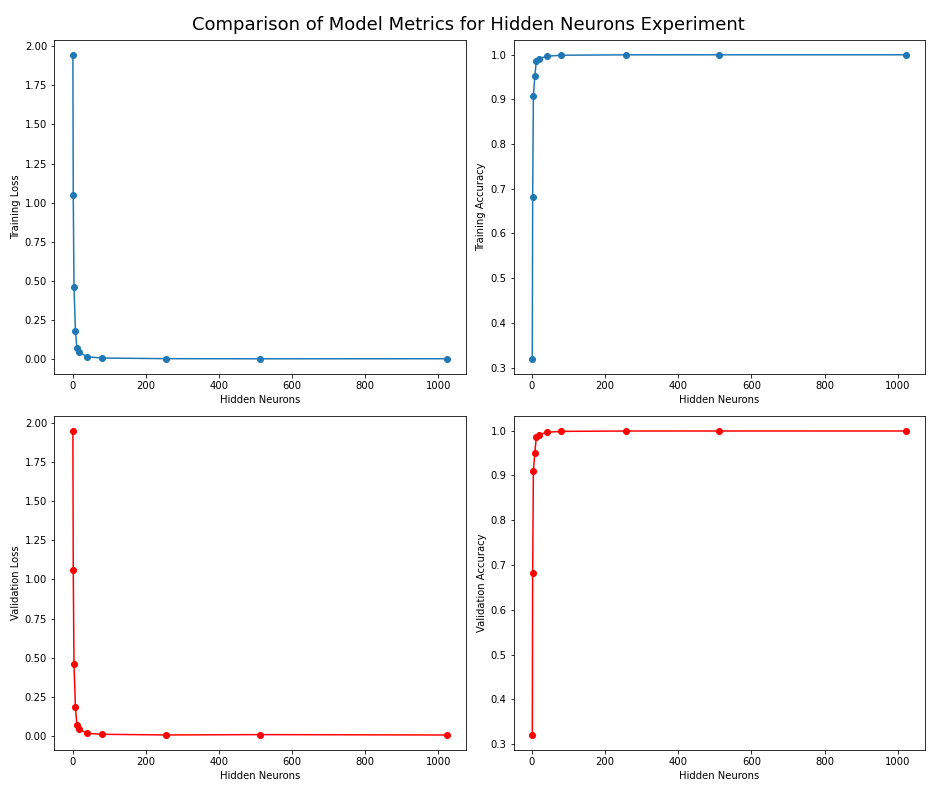
Loss function and accuracy for hidden neurons for last epoch

Figure: The model’s loss and accuracy for both the training and validation datasets as a function of the number of hidden neurons.

Below is the code for visualizing the post-analysis as a bar graph.

Discussion: Are there any other methods of analyzing the data graphically? What are the use cases?

#Helper functions

def create_bar_chart(xData, df, typeOfExperiment, addSaveTitle="", show=True, combined=False):
    """ Create a bar chart using the combined boolean to determine whether to plot 
    the training and validation accuracy vs. type of experiment or to combine it with the
    the training and validation loss vs. type of experiment plot.
    
    Args:
        xData: the x-axis data labels
        df (dataFrame): the DataFrame that holds the accuracy and/or loss.
        typeOfExperiment (string): the type of experiment type. This is used to define the title and x-axis labels.
        addSaveTitle (string): the additional string to add to the save file name.
        show (boolean): whether to show and save the plot.
        combined (boolean): whether to plot the combined loss and accuracy plots or just the accuracy plot. 
    """
    if combined:
        # Initalize the subplots
        fig, ax = plt.subplots(nrows=1, ncols=2, figsize=(15, 10))
        # define the width and positions
        bar_width = 0.15
        bar_positions = range(len(df))
        
        # create the loss and val_loss bar graph
        ax[0].bar([pos - 2*bar_width for pos in bar_positions], df['loss'], \
                  width=bar_width, label='Loss')
        ax[0].bar([pos - bar_width for pos in bar_positions], df['val_loss'], \
                  width=bar_width, label='Val Loss')
        
        # Set x-axis ticks and labels
        ax[0].set_xticks(bar_positions)
        ax[0].set_xticklabels(xData)
        ax[0].legend() # Add legend
        
        # Set title and labels
        ax[0].set_title('Comparison of Model Loss for ' + typeOfExperiment +' Experiments')
        ax[0].set_xlabel(typeOfExperiment)
        ax[0].set_ylabel('Loss')
        
        # add the accuracy bar chart
        create_accuracy_bar_chart(xData, df, typeOfExperiment, fig, ax[1], addSaveTitle=addSaveTitle, show=True)
        
    else:
        # Initalize the subplots
        fig, ax = plt.subplots(figsize=(15, 10))
        # create the accuracy bar chart
        create_accuracy_bar_chart(xData, df, typeOfExperiment, fig, ax, addSaveTitle=addSaveTitle, show=True)

        
def create_accuracy_bar_chart(xData, df, typeOfExperiment, fig, ax, show=True, addSaveTitle=""):
    """ Create the accuracy bar chart.
    
    Args:
        xData: the x-axis data labels
        df (dataFrame): the DataFrame that holds the accuracy and/or loss.
        typeOfExperiment (string): the type of experiment type. This is used to define the title and x-axis labels.
        fig (Figure): the figure object for the plot.
        ax (Axes): the axis object to use to plot.
        show (boolean): whether to show and save the plot.
        addSaveTitle (string): the additional string to add to the save file name. 
    """
    # Set the width and height of the bar chart
    bar_width = 0.15
    bar_positions = range(len(df))

    # Create the accuracy and val_accuracy bar graph
    ax.bar(bar_positions, df['accuracy'], width=bar_width, label='Accuracy')
    ax.bar([pos + bar_width for pos in bar_positions], df['val_accuracy'], \
            width=bar_width, label='Val Accuracy')

    # Set x-axis ticks and labels
    ax.set_xticks(bar_positions)
    ax.set_xticklabels(xData)
    # Add legend
    ax.legend()
    # Set title and labels
    ax.set_title('Comparison of Model Accuracy for ' + typeOfExperiment+' Experiments')
    ax.set_xlabel(typeOfExperiment)
    ax.set_ylabel('Accuracy')

    # Additional formating
    plt.tight_layout()
    
    # adjust the save file name
    typeOfExperiment1 = typeOfExperiment.replace(" ", "_")
    fig = plt.gcf()
    # save and show the plots
    if show:
        plt.savefig("Post_Analysis_"+typeOfExperiment1+"_Experiment"+ addSaveTitle +"_Bar_Graph.png")
        plt.show()

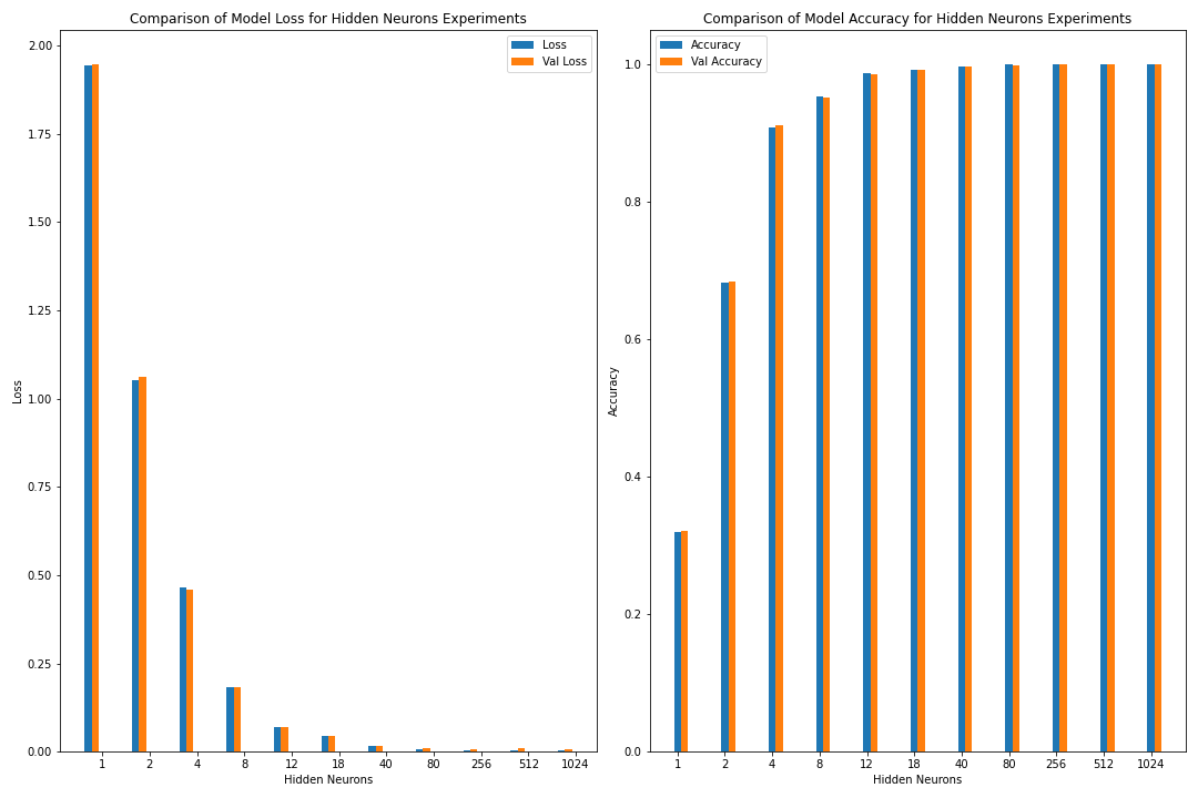
Loss function and accuracy for hidden neurons for last epoch

Figure: The model’s loss and accuracy for both the training and validation datasets as a function of the number of hidden neurons (as a bar graph).

What Did We Learn from the Tuning Experiments Part 1?

Let us recap what we learned from this experiments by answering the following questions:

What happened to the model’s accuracy when we reduce the hidden_neurons hyperparameter? Describe the change in the accuracy of the model as we reduce the hidden_neurons hyperparameter to an extremely small number.

What happened to the accuracy if we increase the hidden_neurons hyperparameter? Discuss (or observe) what would happen if the hidden layer contains 1,000 or even 10,000 hidden neurons?

In conclusion: In order to improve the accuracy of the model, should we use more or less hidden neurons?

Solutions

When the number of hidden neurons in a model is reduced, a discernible trend begins to emerge in the accuracy of the model. Initially, a modest reduction in the hidden layer resulted in moderately worse accuracy. Reducing the number of hidden neurons to extremely low numbers leads to a significant damage in the model’s accuracy. This marked drop-off signifies that the model’s capacity to learn complex patterns and nuances within the data has been significantly curtailed. With too few neurons, the model becomes overly simplistic, unable to adequately represent the diversity and intricacies present in the dataset, leading to a substantial deterioration in predictive performance.

Increasing the number of hidden neurons (from the baseline 18) increases the accuracy. Increasing the number of neurons increases the complexity of the model and computation time required.

In conclusion: While adding hidden neurons initially seems promising to improve accuracy, there is a point of diminishing returns beyond which the cost of improvements to accuracy outweighs the slight benefits to the model’s performance. In addition, increasing the number of hidden neurons may decrease due to overfitting or practical limitations. Finding the right balance in the number of hidden neurons is critical to achieving optimal model performance.

DISCUSSION:

What is an optimal value of hidden_neurons that will yield the desirable level of accuracy? For example, what is the value of hidden_neurons that will yield a 99% model accuracy? How about 99.5% accuracy? Can we reach 99.9% accuracy? Keep in mind that neural network model training is very expensive; increasing this hyperparameter may not improve the model significantly!

Importance of Filtering

Filtering is an important tool when doing post-analysis. It allows us to refine the results and only focus on a specific subset. This can allow for exploration of a hypothesis, deepening insights on the data, or filter data that is no longer relevant.

To find a more exact range/location for the point of diminishing return, we will filter the data to only show ≥ 18 hidden neurons.

This investigation should lead us to the conclusion that improvements to the model’s accuracy does not significantly increase after 80 neurons.

Modify the Post-Analysis to Only Show >= 18 neurons.

Modify the post-analysis to only show >= 18 neurons. Also, remove the loss information and only show the accuracy and val_accuracy metrics. This is because the loss visualization was already validated in the post-processing phase (i.e. the loss graphs did not show any abnormal behavior). The post-analysis phase focuses on performance metrics, in this case, accuracy and validation accuracy.

# filter the df_hn DataFrame where the index (column) values are greater than
# or equal to 18
if "neuron" in df_HN.index.name:
    # Since the index is the number of hidden neurons, we can filter the index by 
    # values >= 18 
    df_HN_gr_18 = df_HN[df_HN.index >= 18] 
    # xData will be x-axis data
    xData_HN_gr_18 = df_HN_gr_18.index
    print("Filtered DataFrame of hidden neurons >= 18")
    print(df_HN_gr_18)
    
else:
    # if the hidden_neurons are input as a list
    if "[" in str(df_HN['hidden_neurons'][0]):
        # temporarily remove the "[]" and make it into an integer
        df_HN['hidden_neurons'] = df_HN['hidden_neurons'] \
        .str.replace('[^0-9]', '', regex=True).astype('int32')
    # Filter the 'hidden_neurons' column for values that are >= 18
    df_HN_gr_18 = df_HN[df_hn['hidden_neurons'] >= 18]
    xData_HN_gr_18 = df_HN_gr_18['hidden_neurons'] 
    print("Filtered DataFrame of hidden neurons >= 18")
    print(df_HN_gr_18)

Filtered DataFrame of hidden neurons >= 18
                    loss  accuracy  val_loss  val_accuracy
hidden_neurons                                            
18              0.045203  0.990570  0.043723      0.990589
40              0.016035  0.996434  0.017410      0.996375
80              0.007796  0.998654  0.011362      0.998425
256             0.003840  0.999515  0.007077      0.999194
512             0.002919  0.999606  0.009277      0.999249
1024            0.003308  0.999593  0.006825      0.999231

create_plots(xData_HN_gr_18, df_HN_gr_18, "Hidden Neurons", logScale=False, addSaveTitle="_Gr18", show = True, combined=False, addTitle=">= 18")

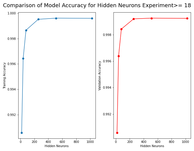
Accuracy for hidden neurons >=18 for last epoch

Figure: The model’s accuracy for both the training and validation datasets as a function of the number of hidden neurons where the number of neurons is greater than or equal to 18.

Deciding an Optimal Hyperparameter, Experiment 1: Varying Hidden Neurons

The example above shows a common theme with model tuning. The more neurons we train, the more accuracy we can achieve (subject to risk of overfitting, see below). You should have observed that at large enough hidden_neurons, the model accuracy started to level off (i.e. adding more neurons will not give significant gain in accuracy).

Since training a neural network model is very expensive, we often have to make a trade-off between doing more trainings (which can be very costly, so may not be possible), and conserving effort against “point of diminishing return,” i.e., the point where improving the model does not yield a significant benefit in the model’s accuracy.

This depends on the application. In some application we may really want to get as close as possible to 100%, then we have no choice but to train more (bite the bullet).

Where is the Point of Diminishing Return for this Experiment?

Can we find this point?

Solution

Improvements to the model’s accuracy does not significantly increase after about 80 neurons.

Takeaways from Tuning Experiments Part 2: Varying Learning Rate

In the second experiment above, we tuned the NN_Model_1H model by varying the learning_rate hyperparameter. Recall that the learning rate hyperparameter determines the step size. In other words, it determines the amount that the model is able to change after each iteration.

Run the post-analysis for the learning rate experiment.

path = 'post_processing_hpc_lr.csv' # path to episode 7's post-processing CSV file 
# path = 'post_processing_hpc_lr_ext.csv' # path to load_bulk_final_metrics CSV file from episode 7
# path = '../model_tuning/post_processing_lr.csv' # path to CSV file from episode 6

df_LR = pd.read_csv(path, index_col=0) # read in the csv file and ignore the additional numbered column

print(df_LR) # print this DataFrame

## Further analysis:
## You can also do things, such as sorting (by one of the result columns, such as loss)
print("\nSorted by val_accuracy:")
print(df_LR.sort_values(['val_accuracy'], ascending=False))

# This is redundant for the post-processing CSV file used in episode 7.
# However, if you utilize the more advanced CSV file creation, you need this.
# This groups the rows by the learning rate value.
# Since this will be unique for each model, we can
# take the last value, which will be the last epoch.
df_LR =  df_LR.groupby('learning_rate').tail(1)

                   loss  accuracy  val_loss  val_accuracy
learning_rate                                            
0.0010         0.018579  0.995926  0.021447      0.995862
0.0100         0.021298  0.995395  0.024532      0.995386
0.0003         0.045203  0.990570  0.043723      0.990589
0.1000         0.444514  0.921821  0.340468      0.921012

Similar to the hidden neurons experiment, we will create visualizations/graphics.

# The following is to accommodate for either type of post-processing CSV file
# The basic type, where the hyperparameter name is the index's name

if "learning_rate" in df_LR.index.name:
    xData_LR = df_LR.index
else:
    # the x-axis data will be the learning rate
    xData_LR = df_LR['learning_rate'] 

# plot the training accuracy vs. learning rate and plot validation accuracy vs. learning rate
create_plots(xData_LR, df_LR, "Learning Rate", logScale=True, addSaveTitle="", show = True, combined=False, addTitle="")

# Create the bar chart for the learning rate experiment.
create_bar_chart(xData_LR, df_LR, "Learning Rate", addSaveTitle="", show=True, combined=False)

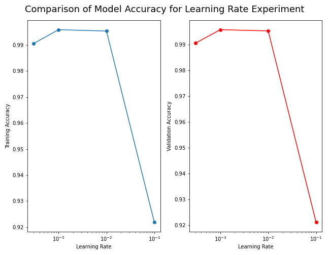
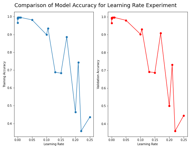
Loss function and accuracy for learning rate for last epoch

Figure: The model’s accuracy for both the training and validation datasets as a function of the learning rate.

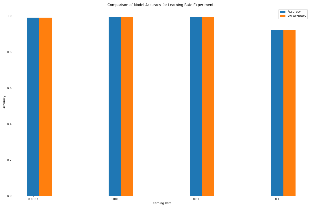
Loss function and accuracy for learning rate for last epoch bar graph

Figure: The model’s accuracy for both the training and validation datasets as a function of the learning rate (as a bar graph).

What did we learn from the Tuning Experiments Part 2?

Answer the questions below to recap what we learn about the effects of the learning rate.

1) What do you observe when we train the network with a small learning rate?

2) What happens to the training process when we increase the learning rate?

3) What happens to the training process when we increase the learning rate even further (to very large values)? Try a value of 0.1 or larger if you have not already.

4) What value of learning rate would you choose, and why?

ANSWERS:

1) When the learning rate is small, the updates to the weights and biases are small. This may cause the training process to converge slowly, requiring more iterations to achieve good results.

2) When the learning rate is large, the update magnitude of weights and biases increases, which can lead to faster training, up to a certain value of learning rate.

3) Beyond this sweet spot, oscillations or instability may occur during training, or even failure to converge to a good solution. Learning rate of 0.01 seems to be good, but the validation accuracy shows an oscillation toward the latter epochs. Learning rates of 0.1 or larger are indeed not good.

Figure: The model’s accuracy for both the training and validation datasets as a function of the learning rate for learning rates greater than 0.1.

4) Important Takeaway: Choosing an appropriate learning rate is one of the key factors when training a neural network, and it needs to be adjusted and optimized according to specific problems and experimental results.

Takeaways from Tuning Experiments Part 3: Varying Batch Size

In the third experiment, we tuned the NN_Model_1H model by varying the batch_size hyperparameter. Recall that batch size is the number of training samples used (in one iteration) to update the model’s parameters.

Run the post-analysis for the batch size experiment.

path = 'post_processing_hpc_bs.csv' # path to episode 7's post-processing CSV file 
# path = 'post_processing_hpc_bs_ext.csv' # path to load_bulk_final_metrics CSV file from episode 7
# path = '../model_tuning/post_processing_bs.csv' # path to CSV file from episode 6

df_BS = pd.read_csv(path, index_col=0) # read in the csv file and ignore the additional numbered column

print(df_BS) # print this DataFrame

## Further analysis:
## You can also do things, such as sorting (by one of the result columns, such as loss)
print("\nSorted by val_accuracy:")
print(df_BS.sort_values(['val_accuracy'], ascending=False))

# This is redundant for the post-processing CSV file used in episode 7.
# However, if you utilize the more advanced CSV file creation, you need this.
# This groups the rows by the batch size value.
# Since this will be unique for each model, we can
# take the last value, which will be the last epoch.
df_BS =  df_BS.groupby('batch_size').tail(1)

                loss  accuracy  val_loss  val_accuracy
batch_size                                            
16          0.023600  0.994557  0.023432      0.994763
32          0.045203  0.990570  0.043723      0.990589
128         0.071049  0.985741  0.070776      0.985224
64          0.062618  0.985123  0.064284      0.984968
512         0.164543  0.959549  0.161178      0.959133
1024        0.276155  0.930404  0.273338      0.931119

Similar to the experiments above, we will create visualizations.

# The following is to accommodate for either type of post-processing CSV file
# The basic type, where the hyperparameter name is the index's name

if "batch_size" in df_BS.index.name:
    xData_BS = df_BS.index
else:
    # the x-axis data will be the batch size
    xData_BS = df_BS['batch_size']    

# plot the training accuracy vs. learning rate and plot validation accuracy vs. batch size
create_plots(xData_BS, df_BS, "Batch Size", logScale=True, addSaveTitle="", show = True, combined=False, addTitle="")

# Create the bar chart for the batch size experiment.
create_bar_chart(xData_BS, df_BS, "Batch Size", addSaveTitle="", show=True, combined=False)

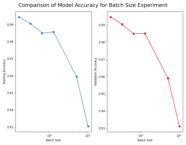
Loss function and accuracy for batch size for last epoch

Figure: The model’s accuracy for both the training and validation datasets as a function of the batch size.

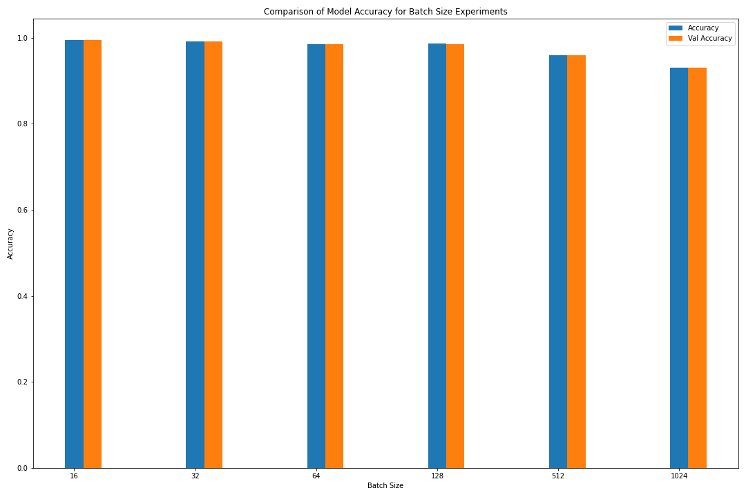
Loss function and accuracy for batch size for last epoch bar graph

Figure: The model’s accuracy for both the training and validation datasets as a function of the batch size (as a bar graph).

What did we learn from the Tuning Experiments Part 3?

Answer the questions below to recap what we learn about the effects of the learning rate.

1) What do you observe when the batch size changes?

2) How do you choose the right batch size?

ANSWERS:

1) As the batch size increases, although the training time is shortened, the accuracy rate decreases. This decrease in accuracy is more obvious with the results from the 1st lesson, where a batch size change from 16 to 1024 causes the validation accuracy to drop from 0.981 to 0.7573.

2) Common batch size choices are powers of 2 (e.g., 32, 64, 128, 256) due to hardware optimizations. However, there is no one-size-fits-all answer. It depends on the specific problem, dataset, model architecture, and available resources.

Takeaways from Tuning Experiments Part 4: Varying the Number of Hidden Layers

In the fourth experiment, we tuned the NN_Model_1H model by varying the number of hidden layers hyperparameter (the number of hidden neurons in each layer still remain 18). Recall that the number of hidden layers is usually referred to as the depth of the model. More hidden layers increases the computational time. It also increases the capability of the model to learn more complex patterns.

Run the post-analysis for the multiple layer experiment.

path = 'post_processing_hpc_layers.csv' # path to episode 7's post-processing CSV file 
# path = 'post_processing_hpc_lauers_ext.csv' # path to load_bulk_final_metrics CSV file from episode 7
# path = '../model_tuning/post_processing_layers.csv' # path to CSV file from episode 6

df_HL = pd.read_csv(path, index_col=0) # read in the csv file and ignore the additional numbered column

print(df_HL) # print this DataFrame

## Further analysis:
## You can also do things, such as sorting (by one of the result columns, such as loss)
print("\nSorted by val_accuracy:")
print(df_HL.sort_values(['val_accuracy'], ascending=False))

# This is redundant for the post-processing CSV file used in episode 7.
# However, if you utilize the more advanced CSV file creation, you need this.
# This groups the rows by the hidden neurons per layer value.
# Since this will be unique for each model, we can
# take the last value, which will be the last epoch.
df_HL =  df_HL.groupby('hidden_neurons').tail(1)

                      loss  accuracy  val_loss  val_accuracy
neurons
[18, 18]          0.011239  0.997849  0.012328      0.997894
[18, 18, 18]      0.016116  0.996846  0.019097      0.997016
[18, 18, 18, 18]  0.018118  0.995839  0.020112      0.995130
[18]              0.043249  0.990277  0.043251      0.989911

Let’s create the visualizations.

# The following is to accommodate for either type of post-processing CSV file
# The basic type, where the hyperparameter name is the index's name

if "neuron" in df_HL.index.name:
    xData_HL = df_HL.index
else:
    # if the hidden_neurons are input as a list
    if "[" in str(df_HL['hidden_neurons'][0]):
        # temporarily remove the "[]" and make it into an integer
        df_HL['hidden_neurons'] = df_HL['hidden_neurons'] \
        .str.replace('[^0-9]', '', regex=True).astype('int32')        
    # the x-axis data will be the hidden neurons
    xData_HL = df_HN['hidden_neurons']    

# plot the training accuracy vs. learning rate and plot validation accuracy vs. multiple hidden layers
create_plots(xData_HL, df_HL, "Multiple Hidden Layers", logScale=False, addSaveTitle="", show = True, combined=False, addTitle="")

# Create the bar chart for the multiple hidden layers experiment.
create_bar_chart(xData_HL, df_HL, "Multiple Hidden Layers", addSaveTitle="", show=True, combined=False)

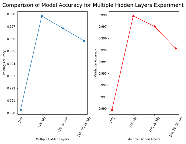
Loss function and accuracy for layer for last epoch

Figure: The model’s accuracy for both the training and validation datasets as a function of the number of hidden layers.

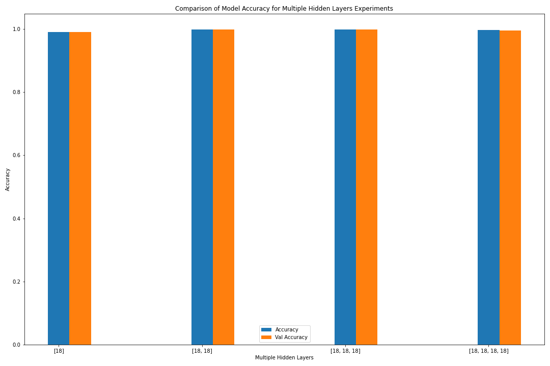
Loss function and accuracy for layer for last epoch

Figure: The model’s accuracy for both the training and validation datasets as a function of the number of hidden layers (as a bar graph).

What did we learn from the Tuning Experiments Part 4?

Answer the questions below to recap what we learn about the effects of the number of hidden layers.

1) How many neurons should be in each hidden layer?

2) What did you observe?

3) What do we learn from here?

ANSWERS:

1) The number of neurons to use in each hidden layer is problem dependent. It will take more experiments to determine the optimal number of neurons in each hidden layer.

2) The model with the least number of layers, and thus the least complex, performs the worst, according to the validation accuracy. The model with four layers performed the second to the worst, according to the validation accuracy. This is the type of experiment where we need to consider the point of diminishing return. Does the increased accuracy of the model between one and three hidden layers outweigh the additional computational cost?

3) Usually, the more neurons we train, the more accuracy we can get (subject to risk of overfitting, vanishing and exploding gradients).
While increasing the number of hidden layers in a neural network can potentially improve its ability to learn complex patterns and representations, it does not guarantee higher accuracy.

Summary

Post-analysis of both episodes lead us to the following conclusions about each of the hyperparameters.

1) Hidden Neurons Experiment: Increasing the number of hidden neurons increases the complexity of the model. This increases the accuracy of the model, until point of diminishing return, when the improvement is deemed not significant (especially compared to the additional time required). Or until the accuracy decreases due to overfitting or practical limitations.

2) Learning Rate Experiment: Smaller learning rates converge slower, since the change in the parameters are smaller, requiring more iterations. Larger learning rates train faster, but might overshoot the optimal answer. Very large learning rates will cause oscillations or instability. Typically a small value is ideal, for this experiment, 0.01 or even 0.001 are good.

3) Batch Size Experiment: Increasing the batch size decreases the accuracy, but shortens the training time.

4) Mulitple Hidden Layer Experiment: This hyperparameter is very problem dependent. Increasing the number of hidden layers increases the model’s complexity and thus capability to learn more complex problems. However, it does not guarantee higher accuracy, as demonstrated in this experiment by the model with four hidden layers not performing as well as one with two.

Post-Analysis-general-rules

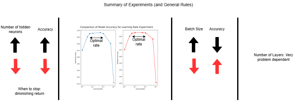
Figure: Post-analysis summary for the experiments (general rules).

Key Points

Post-analysis focuses on analyzing the results (of a model) to better understand the behavior and improve its performance.

previous episode

DeapSECURE module 4: Deep Learning (Neural Network)

next episode

Post-Analysis for Modeling Tuning Experiments

Overview

Introduction

The Baseline Model

Goals of Post-Analysis

Conceptual Aside

Takeaways from Tuning Experiments Part 1: Varying Hidden Layers

Visualizing the results

Note:

Step 0: Import Modules

Step 2: Creating the Visualizations:

What Did We Learn from the Tuning Experiments Part 1?

Solutions

DISCUSSION:

Importance of Filtering

Modify the Post-Analysis to Only Show >= 18 neurons.

Deciding an Optimal Hyperparameter, Experiment 1: Varying Hidden Neurons

Where is the Point of Diminishing Return for this Experiment?

Solution

Takeaways from Tuning Experiments Part 2: Varying Learning Rate

What did we learn from the Tuning Experiments Part 2?

ANSWERS:

Takeaways from Tuning Experiments Part 3: Varying Batch Size

What did we learn from the Tuning Experiments Part 3?

ANSWERS:

Takeaways from Tuning Experiments Part 4: Varying the Number of Hidden Layers

What did we learn from the Tuning Experiments Part 4?

ANSWERS:

Summary

Key Points

previous episode

next episode